Hello, welcome to this customer churn analysis report. If you’ll be following allowing with the code, the csv file needed can be found on Kaggle.com or at https://github.com/BrandonSmith710/customerChurnAnalysis. Click on the filename reading, “churn.csv” and then click download. Then, you’ll just need to make sure the necessary requirements are installed in your environment(category_encoders==2.*, pdpbox==0.2.1, imgaug==0.2.5).
In this report, we will analyze independent variables of the dataset for a couple of purposes. We will see the distributions of both dependent and independent variables, preprocess the data for machine learning, train a number of ML/AI models on the data, investigate independent variables and their continuum of impact on ML model performance scores, optimize a random forest classifier model with a hyperparameter gridsearch, and finally report each model’s performance.
import warnings
warnings.filterwarnings("ignore", category = FutureWarning)
import pandas as pd
import numpy as np
from sklearn.ensemble import RandomForestClassifier
from sklearn.model_selection import train_test_split, GridSearchCV
from sklearn.model_selection import cross_val_score
from sklearn.linear_model import LogisticRegression
from sklearn.metrics import accuracy_score, confusion_matrix
from sklearn.metrics import classification_report, roc_curve, f1_score
from sklearn.impute import KNNImputer
from sklearn.neighbors import KNeighborsClassifier
from xgboost import XGBClassifier
from sklearn.linear_model import LogisticRegression
from category_encoders import OrdinalEncoder
from sklearn.preprocessing import StandardScaler
from sklearn.pipeline import make_pipeline
import matplotlib.pyplot as plt
import seaborn as sns
from pdpbox import pdp
from sklearn.metrics import ConfusionMatrixDisplay

df = pd.read_csv('churn.csv', parse_dates = ['joining_date'])
df.drop('Unnamed: 0', axis = 1, inplace = True)
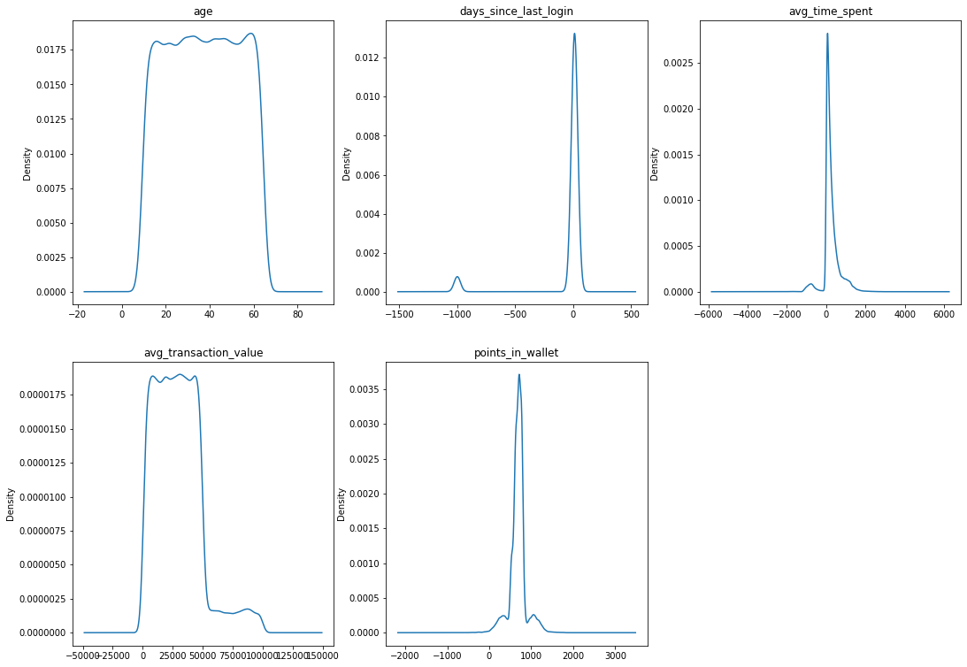
Explore the data: visualize the feature distributions
# first group the numeric features
df_nums = df.drop('churn_risk_score', axis = 1).select_dtypes(include = [int,
                                                                         float]
                  )
plt.figure(figsize = (18, 13))
for i, col in enumerate(df_nums):
    plt.subplot(2, 3, i + 1)
    plt.title(col)
    df_nums[col].plot(kind = 'kde')
# next isolate the categorical variables
df_cats = df.drop(['referral_id','last_visit_time','avg_frequency_login_days',
                      'security_no','joining_date'], axis = 1
                     ).select_dtypes(include = 'object')
plt.figure(figsize = (20, 24))
for i, col in enumerate(df_cats):
    plt.subplot(4, 3, i + 1)
    ax = sns.countplot(x = df_cats[col])
    ax.set_xticklabels(ax.get_xticklabels(), rotation = 35)
    plt.tight_layout()
plt.show()

Plot target distribution
pd.Series([16980, 20012]).plot(kind = 'bar')
plt.show()

Clean and impute missing or unusable data
# several columns contain invalid values which need to be replaced or removed
df['joined_through_referral'] = pd.Series(
    np.nan if i == '?' else i for i in df['joined_through_referral'])
df['gender'] = df['gender'].replace('Unknown', np.nan)
df['medium_of_operation'] = df['medium_of_operation'].replace('?', np.nan)
df['avg_time_spent'] = df['avg_time_spent'].apply(lambda x: x if x >= 0 else
                                                  np.nan)
df['points_in_wallet'] = df['points_in_wallet'].apply(lambda x: x if x >= 0 else
                                                      np.nan)
df['avg_frequency_login_days'] = df['avg_frequency_login_days'].apply(
    lambda x: x if type(x) == float and x >= 0 else np.nan)
df['days_since_last_login'] = df['days_since_last_login'].apply(
    lambda x: x if x >= 0 else np.nan)

# impute null categorical values with mode of the column
for col in '''joined_through_referral gender medium_of_operation
preferred_offer_types region_category'''.split():
    df[col].fillna(df[col].mode()[0], inplace = True)
m_n = df[['points_in_wallet', 'avg_time_spent', 'days_since_last_login']
                 ]
imputer = KNNImputer(n_neighbors = 3)
imputed_values = imputer.fit_transform(m_n)

dft = pd.DataFrame({
    x: imputed_values.T[i] for i, x in enumerate(missing_num.columns)
})
df['year'] = df['joining_date'].apply(lambda x: x.year)
cols2drop = '''internet_option joining_date complaint_status region_category
               preferred_offer_types medium_of_operation gender
               joined_through_referral offer_application_preference
               used_special_discount past_complaint'''.split()

df.drop(['avg_frequency_login_days','points_in_wallet','days_since_last_login',
         'avg_time_spent'] + cols2drop, axis = 1, inplace = True)

df = pd.concat([df, dft], axis = 1)
df = df.drop('security_no referral_id last_visit_time'.split(), axis = 1)
Split data and establish baseline accuracy
target = 'churn_risk_score'
X = df.drop(columns = [target])
y = df[target]
X_train, X_test, y_train, y_test = train_test_split(X, y, random_state = 42,
                                                    test_size = .19)
baseline = [1] * len(y_test)
print('Baseline accuracy', accuracy_score(y_test, baseline))
Baseline accuracy 0.5436050647318253
Encode categorical features
cols2encode = []
for x in df:
    if df[x].dtype == 'object':
        if df[x].nunique() <= 10:
            cols2encode += [x]

ord_enc = OrdinalEncoder(cols = cols2encode)

pipe_rf = make_pipeline(ord_enc,
                        StandardScaler(),
                        RandomForestClassifier(random_state = 42, n_jobs = -1))
Gridsearch for model hyperparameters
- To show the impact of the hyperparameter gridsearch method, only the Random Forest Classifier has been gridsearched for hyperparameters. The other models were fitted using either default values, naive assumption or a combination of the two.
- The Random Forest Classifier would typically place lower than the Extreme Gradient Boosting Classifier in a controlled comparison of accuracies, this is a metric we can use to gauge the impact of our hyperparameter gridsearch. Using only a three-parameter grid, the increase in model performance is apparent.
params_rf = {'randomforestclassifier__max_depth': range(15, 24),
             'randomforestclassifier__max_features': ['auto', 'sqrt'],
             'randomforestclassifier__n_estimators': range(60, 105, 10)}

grid_rf = GridSearchCV(pipe_rf, param_grid = params_rf, n_jobs = -1, cv = 5)
grid_rf.fit(X, y)
grid_rf.best_params_
Below are the parameters output by the gridsearch {‘randomforestclassifier__max_depth’: 15, ‘randomforestclassifier__max_features’: ‘auto’, ‘randomforestclassifier__n_estimators’: 60}
Now it is time to construct the final models which will be compared, these are built using the hyperparameters that were chosen or searched for.
pipe_rf = make_pipeline(ord_enc,
                        StandardScaler(),
                        RandomForestClassifier(max_depth = 15,
                                               max_features = 'auto',
                                               n_estimators = 60,
                                               random_state = 42, n_jobs = -1))
pipe_xgb = make_pipeline(ord_enc,
                         StandardScaler(),
                         XGBClassifier(max_depth = 17, n_estimators = 75,
                                       learning_rate = .0000019, n_jobs = -1,
                                       random_state = 42))
pipe_knn = make_pipeline(ord_enc,
                         StandardScaler(),
                         KNeighborsClassifier(n_jobs = -1, n_neighbors = 8,
                                              weights = 'uniform',
                                              algorithm = 'kd_tree',
                                              leaf_size = 35
                                              ))
pipe_logr = make_pipeline(ord_enc,
                          StandardScaler(),
                          LogisticRegression(n_jobs = -1))

m = 'Random_Forest XGB KNeighbors Logistic_Regression'.split()
cv_rf = cross_val_score(pipe_rf, X, y, n_jobs = -1, cv = 5)
cv_xgb = cross_val_score(pipe_xgb, X, y, n_jobs = -1, cv = 5)
cv_knn = cross_val_score(pipe_knn, X, y, n_jobs = -1, cv = 5)
cv_logr = cross_val_score(pipe_logr, X, y, n_jobs = -1, cv = 5)
l = [cv_rf, cv_xgb, cv_knn, cv_logr]
print('\n'.join(f'{b}: cross validation - {a.mean()}' for a, b in zip(l, m)))
Random_Forest: cross validation - 0.9344452997948292
XGB: cross validation - 0.9300389116830085
KNeighbors: cross validation - 0.8797575138292913
Logistic_Regression: cross validation - 0.7376987771631751
pipe_rf.fit(X_train, y_train)
pipe_xgb.fit(X_train, y_train)
pipe_knn.fit(X_train, y_train)
pipe_logr.fit(X_train, y_train)
importances = pipe_rf.named_steps['randomforestclassifier'].feature_importances_
feats = X_train.columns
pd.Series(data = importances, index = feats
          ).sort_values().tail(15).plot(kind = 'barh')
plt.show()

The feature importances of the model are helpful for investigating features which the model would benefit from an alteration or deletion of.
k = {'Training Acc.': [], 'Test Acc.': [], 'F1 Score': []}
# add the scores to dictionary for later comparison
for name, model in zip(m, [pipe_rf, pipe_xgb, pipe_knn, pipe_logr]):
    k['Training Acc.'] += [model.score(X_train, y_train)]
    k['Test Acc.'] += [model.score(X_test, y_test)]
    k['F1 Score'] += [f1_score(y_test, model.predict(X_test))]
df = pd.DataFrame(k, index = m)
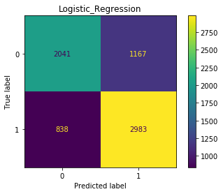
Plot confusion matrices
for name, est in zip(m, [pipe_rf, pipe_xgb, pipe_knn, pipe_logr]):
    ConfusionMatrixDisplay.from_estimator(
        est, X_test, y_test)
    plt.title(name)
plt.show()


Classification Reports - Precision, Recall and F1 Score
for name, est in zip(m, [pipe_rf, pipe_xgb, pipe_knn, pipe_logr]):
    print(name + '\n' + classification_report(y_test, est.predict(X_test)))
Next we will look at the partial dependence of predictor variables for the XGBClassifier
- most notable is the dependence of the points_in_wallet feature
for feat in X_test.drop(columns = ['feedback', 'membership_category',
                                'days_since_last_login']):
 pdp_dist = pdp.pdp_isolate(model = pipe_xgb, dataset = X_test,
                            model_features = X_test.columns, feature = feat)
 pdp.pdp_plot(pdp_dist, feat)
plt.show()


As you can see in the PDP plot for points_in_wallet, the predicted value for churn increases right around 500 points, and decreases right around 700. If you’ll recall the Kernal Density Estimate plots shown in the EDA section of this report, points_in_wallet saw a sharp spike in density right around 500 points, and then a decrease at about 700. It is noticeable that the majority of customers are within the 500-700 range of points_in_wallet, and it is within reason to say that the majority of customers who churn, come from the majority of customers, and that since the majority customers have a points_in_wallet value in the range of 500-700, a typical points_in_wallet range for a customer to churn with would be 500-700.
plt.figure(figsize = (10, 7))
col = 'points_in_wallet'
plt.title(col)
df_nums[col].plot(kind = 'kde')
plt.show()

Plot the ROC Curve for each classifier
plt.figure(figsize = (18, 20))
for i, est in enumerate(zip(m, [pipe_rf, pipe_xgb, pipe_knn, pipe_logr])):
    y_pred_prob = est[1].predict_proba(X_test)[:, 1]
    fpr, tpr, thresholds = roc_curve(y_test, y_pred_prob)
    plt.subplot(2, 2, i + 1)
    plt.plot(fpr, tpr)
    plt.plot([0, 1], ls = '--')
    plt.title(f'ROC curve for {est[0]}')
    plt.xlabel('False Positive Rate')
    plt.ylabel('True Positive Rate')

Compare model scores
#	               Training Acc.    Test Acc.       F1 Score
# Random_Forest	        0.966158	0.933419	0.938695
# XGB	                0.957648	0.922606	0.929716
# KNeighbors	        0.882856	0.849054	0.858778
# Logistic_Regression	0.703801	0.714753	0.748463
Thanks for reading!